Query Optimisation in Databases

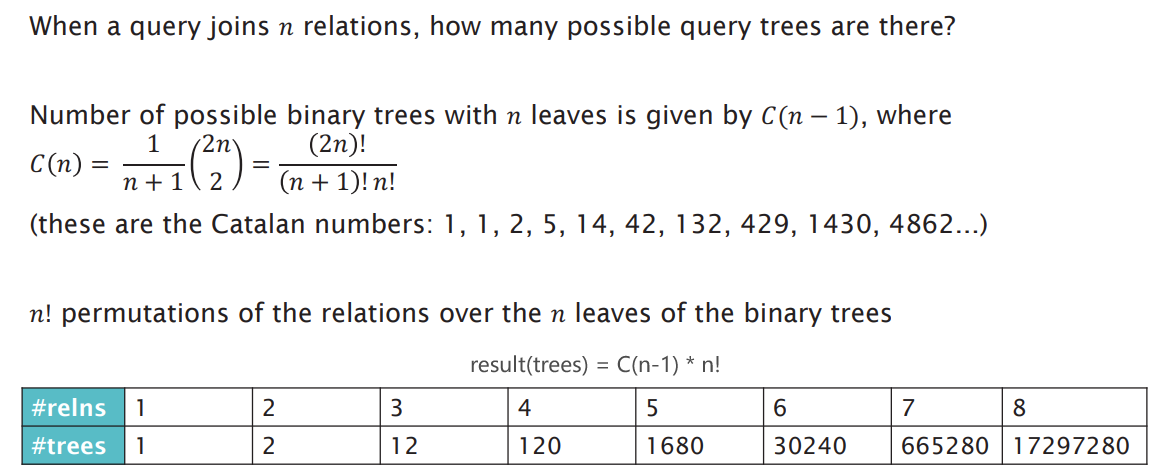
When we know how to do cost estimation, we have a way of determining whether one plan is better than another. Our next step is to compare all possible plans to find the optimal plan.

But here’s the problem: How many possible plans are there?

Contents

How Many Query Trees in a Relational Query?
- The Main Determinant of Query Cost: Joining Order
Query Graphs
Optimising Query Trees (Optimised Logical Query Plan)
- Optimisation Approaches
- Example (Heuristic)

How Many Query Trees in a Relational Query?

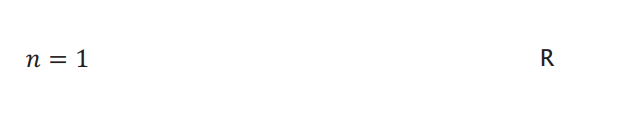
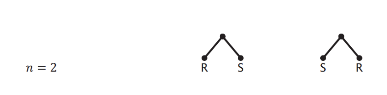
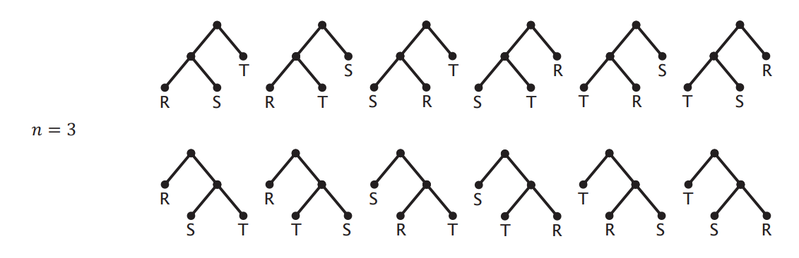
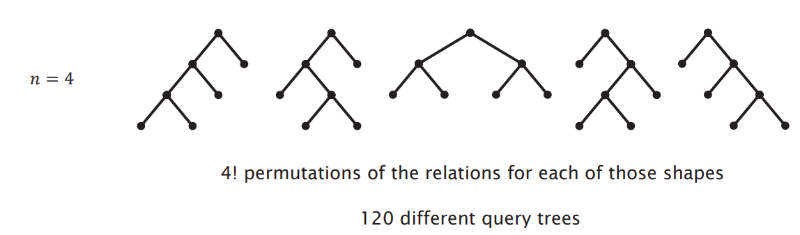
Considering plans with only × or ⋈, and with n relations:

The Main Determinant of Query Cost: Joining Order

As above, the number of query trees explodes with increasing of n (number of relations)
So, in reality, it is impossible to perform an exhaustive search to determiner which query tree is best (which query plan is best).
Join ordering is the main determiner of query cost
- Need to use Query Graphs to guide search through space of possible join orderings
- Prefer ⋈ over × (smaller output relation, which is cheaper)

Query Graphs

Example

For this example, we consider conjunctive queries with simple predicates only (i.e. predicates of the form a = b or a = 1)
Queries join base relations R1, R2, ..., Rn, possibly modified by selections
We can construct a query graph for queries of this type
- Undirected graph
  - Undirected graphs are used because the connections between relationships are usually bi-directional, which means that the order of the connections can be arbitrary and does not affect the final result. (Join operations don’t care about the order)
- Vertices (R1, R2, ..., Rn)
- Edges (<R, S>)
  - A predicate of the form a = b, where a ∈ R1 and b ∈ R2, gives an edge <R1, R2>
  - A predicate of the form a = 1, where a ∈ R1, gives an edge <R1, R1>

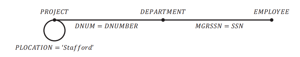
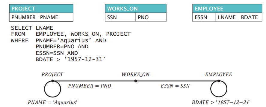
Assuming, we have the following 3 tables:

        
      
SELECT PNUMBER, DNUM, LNAME, ADDRESS, DATE
FROM PROJECT, DEPARTMENT, EMPLOYEE
WHERE DNUM=DNUMBER AND MGRSSN=SSN AND PLOCATION='Stafford'

For the above SQL, we can get the following undirected graph:

Different Query Graphs

Query graph shapes

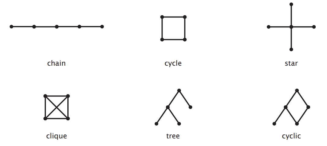
Different query graph structures serve specific use cases:
- Chain: When a query involves several tables, and each table is joined only with the previous and/or next table in the chain, a chain structure is formed.
- Cycle: A cycle structure emerges in a query graph when the join conditions create a closed loop among the tables. This means that starting from one table, you can follow the join conditions through a series of tables and eventually return to the starting table.
- Star: When there is a central fact table surrounded by multiple dimension tables connected to it, a star structure is formed. This is common in star schema data warehouses.
- Clique: When a query requires multiple tables and each table must be joined with every other table, a clique structure is formed. This typically occurs in query designs that require a full join among multiple tables.
- Tree: When a query can be executed without forming any cycles, meaning no table needs to be joined twice, a tree structure is formed.
- Cyclic: When the join relations in a query contain cycles, a cyclic structure is formed. This might require more optimization to reduce the cost of the query.
They can help us exclude join orderings that would lead to cross products (Cross products/joins, which is ×, means that every row in two tables matches every row in another table once, resulting in a result set whose size is the product of the number of rows in the two tables. Cross products/joins tend to be very inefficient because they generate a lot of unnecessary data).

Join Trees

Choice of join tree shapes also constrains search space
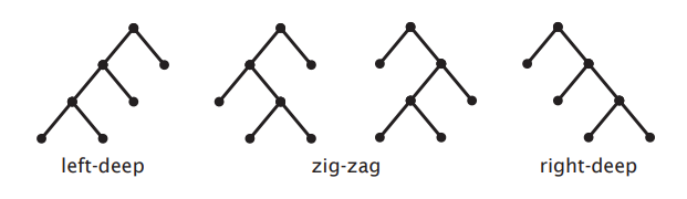
Two main classes of join tree
- Linear (left-deep, right-deep, zig-zag)
- Bushy
Choice depends on:
- Algorithms chosen (i.e. physical plan operators)
- Execution model

Linear Join Trees

Every join introduces at least one base relation
Better for pipelining - avoids materialisation
Possible left-deep trees: n!
Possible right-deep trees: n!
Possible zig-zag trees: n! * 2^(n-2)

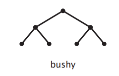
Bushy Join Trees

Some joins may not join any base relations
Need not be balanced
Better for parallel processing
Possible bushy trees: n! * C(n-1) = (2n)!/n!
Linear Join Trees is a special type of Bushy Join Trees

Optimising Query Trees (Optimised Logical Query Plan)

Optimisation Approaches

Wide variety of approaches (no single best approach)
- Heuristic: transformation rules, keep transformed plan if cheaper
  1. Start with canonical form
  2. Push σ operators down the tree
  3. Introduce joins (combine × and σ to create ⋈)
  4. Determine join order
  5. Push π operators down the tree
- Dynamic programming
- Randomised: avoid local minima by randomly jumping within big search spaces
- …

Example (Heuristic)

Transforms into Left-Deep Tree

Query trees should be:
- Useful to only consider left-deep trees (Left-deep trees are easier to translate into efficient execution plans, because the database query optimiser executes the leftmost table joins first)
- Fewer possible left-deep trees than possible bushy trees (smaller search space when investigating join orderings)
- Left deep trees work well with common join algorithms (nested-loop, index, one-pass, …)
Canonical form should be:
- a left-deep tree of products with
- a conjunctive selection above the products and
- a projection (of the output attributes) above the selection

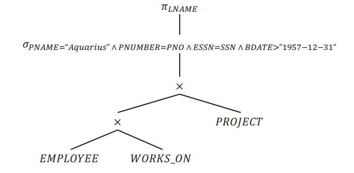Transforms into left-deep tree

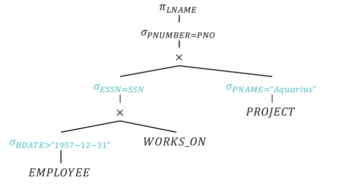
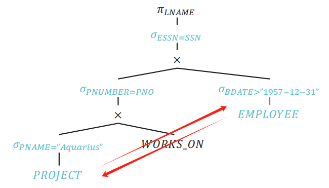
Move `σ` down

According to Relational Transformations σ p∧q∧r (R) = σp(σq(σr(R))) and σp(σq(R)) = σq(σp(R)):
- A selection of the form σ (a = 1) can be pushed down to just above the relation that contains a
- A selection of the form σ (a = b) can be pushed down to the product above the subtree containing the relations that contain a and b

Move σ down

Reorder Joins

If a query joins n relations and we restrict ourselves only to left-deep trees, there are n! possible join orderings
- Far more possible orderings if we don’t restrict to left-deep
For simplicity of search, adopt a greedy approach:
- Reorder subtrees to put the most restrictive relations (fewest tuples) first

Assuming that tuples of PNAME = "Aquarius" is less than BDATE > "1957-12-31":

Reorder Joins

Combine Products to Create joins

According to Relational Transformations σp(R⨉S) = R ⨝p S:
- Combine × with adjacent σ to form ⋈
- Much cheaper than product followed by selection (eliminating a lot of unnecessary data)

Combine 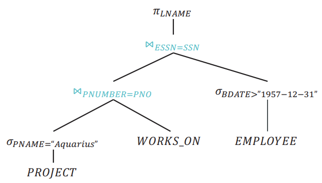Products to Create joins

Move `π` down

If intermediate relations are to be kept in buffers (i.e. materialised), reducing the degree of those relations (number of attributes) allows us to use fewer buffer frames。

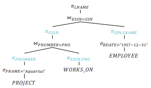Move π down