
When delving into the world of databases, one cannot overlook the fundamental role of relational algebra. It is the backbone of structured query language (SQL), providing a theoretical framework that forms the basis of database operations.
- What is Relational Algebra?
- The Significance of Relational Algebra
- Core Operations and Functions in Relational Algebra
- Multisets (Bags)
- Binary Operations: Join (⨝)
- Relational Transformations
- Relational Algebra and SQL
- Relational Completeness of SQL
What is Relational Algebra?
- An Algebra is a mathematical system consisting of:
- Operands: variables or values from which new values can be constructed
- Operators: symbols denoting procedures that construct new values from the given values
- A Relational Algebra
- Operands: relations or variables that represent relations
- Operators: common things that can be performed on relations
Relational algebra is a set of operations that are used to manipulate and retrieve data stored in relational database structures. It consists of a collection of procedural operations that take one or two relations as input and produce a new relation as output. These operations are mathematical in nature and are similar to those used in traditional set algebra.
- The input of a relational algebra operator is one or more relations
- The result of an operation is always a relation
- Necessary to use relational algebra in a cascaded manner
- Cascaded manner usually refers to a sequential or hierarchical order in which operations or events occur, one after another, often with each step triggering the next.

The Significance of Relational Algebra
Relational algebra is not just an academic concept but is the foundation upon which SQL and other database query languages are built. It provides a formal understanding of how queries are processed and optimized by database management systems (DBMS).
- Understanding relational algebra helps database professionals to:
- Model databases more efficiently.
- Write more effective and optimized queries.
- Understand the internal workings of a DBMS.
- Design and optimize the database schema.
Core Operations and Functions in Relational Algebra
Relational algebra forms the theoretical underpinning of relational databases, providing a systematic way to query and manipulate data using a variety of operations and functions.
 Relations as Subset of a Cartesian Product
Set Operations
Set operations in relational algebra correspond closely to those in mathematical set theory, providing a way to manipulate sets of tuples (rows).
-
Union (∪): Combines the tuples from two relations and eliminates duplicate tuples. Both relations must be union-compatible—meaning they must have the same number of attributes and corresponding attributes must have the same data types.
- Example: If
R1andR2are two relations:R1 ∪ R2will contain all tuples that are inR1,R2, or in both.
- Example: If


-
Difference (-): Generates a set of tuples that are in the first relation but not in the second. Again, the relations involved must be union-compatible.
- Example:
R1 - R2will have tuples that are inR1but not inR2.
- Example:

-
Intersection (∩): Yields tuples that are present in both relations. The relations must be union-compatible for intersection as well.
- Example:
R1 ∩ R2will produce a new set of tuples that are both inR1andR2.R ∩ S = R - (R - S)
- Example:
 R ∩ S = R - (R - S)
-
Cartesian Product (×): Creates a set of combined tuples from two relations, which are not required to be union-compatible.
- Example: If
R1(a1, a2)andR2(b1, b2)are two relations,R1 × R2will result in a new relation with attributes(a1, a2, b1, b2), combining each tuple fromR1with every tuple fromR2.
- Example: If

Commutativity does not hold for Cartesian Product (named or unnamed).
 named
named
 unnamed
-
Set Division (÷): This operation is used when we want to find tuples in one relation (
R1) that are related to all tuples in another relation (R2).- Example: If
R1representsStudentswho are enrolled inCoursesrepresented byR2, thenStudents ÷ Courseswill yield the set of students who are enrolled in all the courses listed inR2.
- Example: If
Relational Database Specific Operations
These operations are more specific to the relational model and are essential for querying databases.
-
Selection (σ): This operation is used to select rows from a relation that satisfy a certain predicate.
- Example:
σ_(age>25)(Employees)would result in a relation containing employees older than 25.
- Example:

- Algebraic laws can be useful in query optimisation
σΘ1(σΘ2(R)) = σΘ1⋀Θ2(R)- Commutative:
σΘ1(σΘ2(R)) = σΘ2(σΘ1(R))σΘ(R⨉S) = σΘ(R) ⨉ S
- if
Θmentions only attributes ofR- Cartesian product is expensive, so reducing the size of
R(σΘ(R) ⨉ S) is beneficial
-
Renaming (ρ): This is used to change the name of attributes in a relation, allowing for clarity or consistency in query results or expressions.
- Example:
ρ B/A (S)returns a relation with schema identical toSbut the attribute nameAhas been replaced byB. E.g. letSwith schemaS(A, B, C, D, E),ρ X/B,Y/D (S)creates a relation with schemaS(A, X, C, Y, E).
- Example:
-
Projection (π): Used to select certain columns from a relation, effectively discarding the other columns.
- Example:
π_(name, salary)(Employees)will create a new relation with just the name and salary columns from theEmployeesrelation.
- Example:


-
Join (⨝): Combines tuples from different relations based on a common attribute.
- Example:
Employees ⨝ Departmentsjoins theEmployeesandDepartmentsrelations on their common attributes (e.g.departmentID).
- Example:

Set Functions
Set functions perform calculations on a set of values and return a single value.
-
sum: Calculates the sum of a numeric attribute over a set of tuples.
- Example:
sum(π_(salary)(Employees))would return the total salary for all employees.
- Example:
-
avg: Computes the average value of a numeric attribute.
- Example:
avg(π_(salary)(Employees))calculates the average salary of employees.
- Example:
-
count: Counts the number of tuples.
- Example:
count(σ_(department='Sales')(Employees))counts the number of employees in the Sales department.
- Example:
-
max: Finds the maximum value of a numeric attribute.
- Example:
max(π_(age)(Employees))returns the age of the oldest employee.
- Example:
-
min: Identifies the minimum value of a numeric attribute.
- Example:
min(π_(age)(Employees))gives the age of the youngest employee.
- Example:
Multisets (Bags)
Sets vs. Multisets (Bags)
- A Multiset (Bag) is like a Set but elements may appear more than once
- Example:
R = {1,3,3,6,6,6,7},S = {1,1,6,6,7}are both multisets
- Example:
- Union of two multisets:
{1,3,3,6,6,6,7} ∪ {1,1,6,6,7} = {1,1,1,3,3,6,6,6,6,6,7,7}
- Difference between two multisets:
{1,3,3,6,6,6,7} - {1,1,6,6,7} = {3, 3, 6}
- Cartesian product:
{1, 3, 3} ⨉ {1, 1, 6} = {<1,1>, <1,1>, <1,6>, <3,1>, <3,1>, <3,6>, <3,1>, <3,1>, <3,6>}
Operations on Multisets (Bags)
Given μ(x, B), defined as the number of occurrences of x in multiset B.
- Union
R ∪ Sμ(t, R ∪ S) = μ(t, R) + μ(t, S)for alltinRandS
- Difference
R – Sμ(t, R – S) = max{μ(t, R) – μ(t, S), 0}for alltinRandS
- Intersection
R ∩ Sμ(t, R ∩ S) = min{μ(t, R), μ(t, S)}for alltinRandS
- Cartesian Product:
μ( tt’, R ⨉ S) = μ(t, R) * μ(t’, S)for alltinRandt’inS
- Projection:
- If
Ris a multiset, thenπX(R)is also a multiset - If
Ris a set, thenπX(R)may be a multiset
- If
- Selection:
- If
Ris a multiset, then the selectionσΘ(R)may be a set - If
Ris a set, then the selectionσΘ(R)is a set
- If
Multisets in SQL
SQL is multiset based.
- Efficiency:
- Duplicate elimination may take quadratic time
- For example, after a projection
- Duplicate elimination may take quadratic time
- Necessity:
- Eliminating duplicates might result in information loss/errors (e.g., in computing averages)
Binary Operations: Join (⨝)
- Binary Operators between two relations
- Used to combine information from two relations into a new relation
- Core to Relational Database
Θ-Join (⨝ F)
- Theta Join combines two relations using a predicate
F:R ⨝F S- It is equivalent to the cartesian product of the two relations followed by a selection using the
predicate:
σF (R⨉S) - It is called a “theta join” because in the original notation,
Θwas used in place ofFand was limited to:=, <, >, <=, >=, != - A theta join that only uses the operator
=is called an Equijoin
- It is equivalent to the cartesian product of the two relations followed by a selection using the
predicate:
 Θ-Join Example
Natural Join (⨝)
- An natural join is a
Θ-joinin which no predicate is specified:R ⨝ S- It is defined an equijoin over all the common attributes of the two relations
- The result contains the common attributes followed by the remaining non-common attributes in
RandS- like an equijoin but the common attributes only appear once
- Natural Join can be formalised as the Cartesian Product of
RandS, followed by the selection on equality amongst the common attributes(A1,.. Ak). Followed by a projection.R ⋈ S = π<list>(σR.A1=S.A1 ⋀ … ⋀ R.Ak = S.Ak (R ⨉ S))- where
- contains
- All the attributes unique to R
- All the common attributes
- All the attributes unique to S
- Given relations:
REGISTERED(student, course, term),TEACHES(lecturer, course, term)- REGISTERED ⋈ TEACHES = TAUGHT(student, course, term, lecturer)
- where
Outer Join (⟕, ⟖, ⟗)
- The Left outer join of two relations
RandSis a natural join which also includes tuples from R which do not have corresponding tuples inS; missing values are set tonullR ⟕ S = R ⋈ S ∪ ((R - πr1, r2,…,rn(R ⋈ S)) ⨉ {<null,…, null>})

- other Outer Join:
- Right Outer Join:
R ⟖ S = ((S – πs1, s2,…,sn(R ⋈ S)) ⨉ {}) ∪ R ⋈ S - Full Outer Join:
R ⟗ S = (((R - πr1, r2,…,rn(R ⋈ S)) ⨉ {}) ∪ ((S – πs1, s2,…,sn(R ⋈ S)) ⨉ {}) ∪ R ⋈ S)
- Right Outer Join:
Right Outer Join (R ⟖ S):
1
2
3
4
5
A    | B | C
-------------
a    | 1 | x
a    | 1 | y
NULL | 3 | z
Full Outer Join (R ⟗ S):
1
2
3
4
5
6
A    | B | C
-------------
a    | 1 | x
a    | 1 | y
b    | 2 | NULL
NULL | 3 | z
- JOIN operations in addition to these outer joins are inner joins.
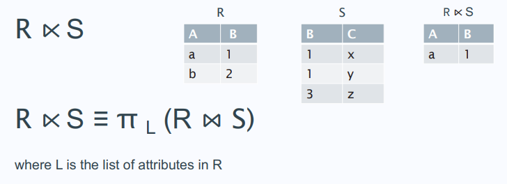
Semijoin (⋉)
- Semijion is like a natural join but the resulting attributes are only taken from
R
Antijoin (▷)
- The antijoin is like semijoin but the result only contains tuples from
Rthat have no match inS

Relational Transformations
- Relational expressions can be transformed with transformation rules
- Used during SQL query optimisation to rewrite user queries
- Database engine aims to improve CPU, memory or disk usage
Relational Transformations - General
- When an expression consists of a series of nested projections, only the last in a sequence of projections is
required:
πLπM…πN(R) = πL(R)- But not if they are extended projections that rely on prior expressions
- If a selection contains a predicate with conjunctive terms (ie ANDs), the terms can cascade into individual
selections
σ p∧q∧r (R) = σp(σq(σr(R)))
σp(R⨉S) = R ⨝p S
Relational Transformations - Commutative
- Selection and theta-join are commutative operations
σp(σq(R)) = σq(σp(R))R ⨝p S = S ⨝p R- But for theta-join, only when using the named perspective
- Selection and projection are commutative
- When an expression consists of a selection followed by a projection, the projection can be done first, if
the selection predicate only involves attributes in the projection list:
-
πA1,…Am(σp(R)) = σp(πA1,…Am (R))
- When an expression consists of a selection followed by a projection, the projection can be done first, if
the selection predicate only involves attributes in the projection list:
-
Relational Transformations - Associativity
- Joins exhibits associativity:
(R ⨝ S) ⨝ T = R ⨝ (S ⨝ T)
Relational Transformations - Distributivity
- Where an expression consists of a theta-join followed by a projection, the selection can be performed on both
relations prior to the theta-join, if the predicate only involves attributes being joined
σp(R ⨝r S) = σp(R) ⨝r σp(S)- In this case, selection distributes over theta-join
- Selection also distributes over set operations
σp(R ∪ S) = σp(R) ∪ σp(S)σp(R ∩ S) = σp(R) ∩ σp(S)σp(R - S) = σp(R) - σp(S)
- Projection distributes over set union
πL(R ∪ S)= πL(R) ∪ πL(S)
- Projection distributes over theta join
π L1 ∪ L2 (R ⨝r S) = πL1(R) ⨝r πL2(S)
Relational Algebra and SQL
| SQL | Relational Algebra |
|---|---|
| SELECT | Projection π |
| FROM | Cartesian Product |
| WHERE | Selection σ |

Example With Selection
DB Schema: FACULTY(name, dpt, salary), CHAIR(dpt, name)
Query: Find the salaries of department chairs
- Relational Algebra:
C-SALARY(dpt,salary) = πF.dpt, F.salary(σF.name = C.name ⋀ F.dpt = C.dpt (FACULTY ⨉ CHAIR))- or
C-SALARY(dpt,salary) = πdpt, salary(FACULTY ⋈ CHAIR)
- SQL:
- SELECT FACULTY.dpt, FACULTY.salary FROM FACULTY, CHAIR WHERE FACULTY.name = CHAIR.name AND FACULTY.dpt = CHAIR.dpt
Example No Selection
Goal: Compute the Cartesian product of relations of S and T
- Relational algebra:
- S ⨉ T
- SQL:
- SELECT * FROM S, T
Example Self-Joins
- Goal: Compute expressions that rely on Self-Joins
- However, relation names in the FROM list must be distinct
- This stops us from computing self-joins, ie FROM R, R
- Many interesting queries involve self-joins
- DB Schema: FATHER(father-name, child-name)
- Compute: GRANDFATHER(grandfather-name, grandchild-name)
Relational Algebra:
- First, take the Cartesian Product of Father and Father
FATHER:
| father-name | child-name |
|---|---|
| David | Nick |
| Nick | Joe |
| Joe | Mick |
FATHER x FATHER:
| father-name | child-name | father-name | child-name |
|---|---|---|---|
| David | Nick | David | Nick |
| Nick | Joe | David | Nick |
| Joe | Mick | David | Nick |
| David | Nick | Nick | Joe |
| Nick | Joe | Nick | Joe |
| Joe | Mick | Nick | Joe |
| David | Nick | Joe | Mick |
| Nick | Joe | Joe | Mick |
| Joe | Mick | Joe | Mick |
- Second, select where the child-name is the same as the father-name:
σ $2=$3 ( FATHER x FATHER)
| father-name | child-name | father-name | child-name |
|---|---|---|---|
| David | Nick | Nick | Joe |
| Nick | Joe | Joe | Mick |
- Then,
π$1,$4 (σ $2=$3 ( FATHER x FATHER))
| father-name | child-name |
|---|---|
| David | Joe |
| Nick | Mick |
- Final,
ρ grandfather-name/father-name, grandchild-name/child-name (π$1,$4 (σ$2=$3 (FATHER ⨉ FATHER)))- get: GRANDFATHER(grandfather-name, grandchild-name)
| grandfather-name | grandchild-name |
|---|---|
| David | Joe |
| Nick | Mick |
SQL:
- SQL does not support referencing columns by position number
- Instead, SQL supports an aliasing mechanism
- SELECT R.father-name AS grandfather-name, T.child-name AS grandchild-name FROM FATHER AS R, FATHER AS T WHERE R.child-name = T.father-name
Relational Completeness of SQL
- SQL can express all relational algebra queries
- i.e., it is a relationally complete database query language
- As we saw:
- SELECT DISTINCT …
- FROM …
- WHERE …
- can express Cartesian product, projection, and selection
- SQL has explicit constructs for union and difference:
- Union
R ∪ S: (SELECT * FROM R) UNION (SELECT * FROM S) - INTERSECT
R ∩ S: (SELECT * FROM R) INTERSECT (SELECT * FROM S) - Difference
R – S: (SELECT * FROM R) EXCEPT (SELECT * FROM S)
- Union
- SQL supports these operations: UNION, EXCEPT, INTERSECT, UNION ALL, INTERSECT ALL and **EXCEPT ALL
**. (There may be some differences in specific SQL implementations (e.g. MySQL, PostgreSQL, etc.) or some database
systems may not support specific operators.)
- UNION, INTERSECT and EXCEPT eliminates duplicates! (Set semantics)
- UNION ALL, INTERSECT ALL and EXCEPT ALL does not (Multiset semantics)
