
- Ordered Pairs (↦) and Cartesian Products (×)
- Relations (↔)
- Partial and Total Functions
- Injective and Surjective Functions
- Restriction and Substraction
- Function Overriding
- Relational Inverse
- Relational Composition
Ordered Pairs (↦) and Cartesian Products (×)
- An ordered pair is an element consisting of two parts: a first part and a second part.
- An ordered pair with first part x and second part y is written:
x↦y
- An ordered pair with first part x and second part y is written:
- The Cartesian product of two sets is the set of pairs whose first part is in
Sand the second part is inT.- The Cartesian product of S with T is written:
S × T
- The Cartesian product of S with T is written:
Cartesian Products: Definition and Examples

Cartesian Product is a Type Constructor
-
S × Tis a new type constructed from typesSandT. -
Cartesian product is the type constructor for ordered pairs.
Given x ∈ S, y ∈ T, we have x ↦ y ∈ S × T

Sets of Order Pairs
- A database can be modelled as a set of ordered pairs:
directory = { mary ↦ 287573, mary ↦ 398620, john ↦ 829483, jim ↦ 398620 }
directory has type: directory ∈ P(Person × PhoneNum)
Relations (↔)
- A relation is a set of ordered pairs.
- A relation is a common modelling structure, so Event-B has a special notation for it:
T ↔ S = P(T × S)- So we can write:
directory ∈ Person ↔ PhoneNum
- So we can write:
- Do not confuse the arrow symbols:
↔combines two sets to form a set:T ↔ S = P(T × S)↦combines two elements to form an ordered pair:x ↦ y ∈ S × T
Domain and Range
- The domain of a relation
Ris the set of first parts of all the pairs inR, written:dom(R) - The range of a relation
Ris the set of second parts of all the pairs inR, written:ran(R)
| Predicate | Definition |
|---|---|
| x ∈ dom(R) | ∃y · x ↦ y ∈ R |
| y ∈ ran(R) | ∃x · x ↦ y ∈ R |
Relational Image
directory = { mary ↦ 287573, mary ↦ 398620, john ↦ 829483, jim ↦ 398620 }
Relational image examples:
directory[ {mary} ] = { 287573, 398620 }directory[ { john, jim } ] = { 829483, 398620 }
Assume R ∈ S ↔ T and A ⊆ S, the relational image of set A under relation R is written R[A]
| Predicate | Definition |
|---|---|
| y ∈ R[A] | ∃x · x ∈ A ∧ x ↦ y ∈ R |
Partial and Total Functions
Partial Functions (⇸)
Special kind of relation: each domain element has at most one range element associated with it. f ∈ X⇸Y
- To declare
fas a partial function- This says that
fis a many-to-one relation - Each domain element is mapped to one range element:
x ∈ dom(f) ⇒ card( f [{x}] ) = 1 - More usually formalised as a uniqueness constraint:
x ↦ y1 ∈ f∧x ↦ y2 ∈ f⇒y1 = y2
- This says that
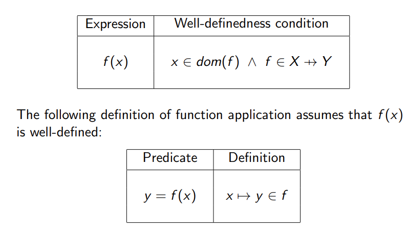
Function Application
We can use function application for partial functions.
- If
x ∈ dom(f), then we writef(x)for the unique range element associated withxinf. - If
x ∉ dom(f), thenf(x)is undefined. - If
card(f [{x}] ) > 1, thenf(x)is undefined.
Example:

Well-definedness
| Predicate | Well-definedness condition |
|---|---|
| f(x) | x ∈ dom(f) ∧ f ∈ X ↦ Y |
The following definition of function application assumes that f(x) is well-defined:
| Predicate | Definition |
|---|---|
| y = f(x) | x ↦ y ∈ f |
In mathematics, a well-defined expression or unambiguous expression is an expression whose definition assigns it a unique interpretation or value. Otherwise, the expression is said to be not well defined, ill defined or ambiguous. A function is well defined if it gives the same result when the representation of the input is changed without changing the value of the input.
Example of Birthday Book
- Birthday book relates people to their birthday.
- Each person can have at most one birthday.
- People can share birthdays.


Total Functions (→)
A total function is a special kind of partial function. To declare f as a total function: f ∈ X → Y.
A total function means that f is well-defined for every element in X, i.e., f ∈ X → Y is shorthand
for f ∈ X⇸Y ∧ dom(f) = X
Total Function: A total function is a function that is defined for every possible input in its domain. For Example:
f(x) = x + 2, where the domain is all real numbers. For every real number you input into this function, you get a valid output (another real number).Partial Function: A partial function, on the other hand, is only defined for some inputs in its domain. For Example:
f(x) = 1/x, where the domain could be considered as all real numbers. However, this function is not defined for the input x = 0 (since division by zero is undefined).
Example of Modelling with Total functions
We can re-write the invariant for the birthday book to use total functions:


Injective and Surjective Functions
Injective Functions (⤔)
One-to-one function: different domain elements are mapped to different range elements. In other words, in inverse is also a function.
To declare f as an (partial) injective function: f ∈ X ⤔ Y
This is defined in terms of the inverse of f as follows:
| Predicate | Definition |
|---|---|
| f ∈ X ⤔ Y | f ∈ X ⇸ Y ∧ f⁻¹ ∈ Y ⇸ X |
Total Injective Functions (↣)
Just as for standard total functions, we can declare an injective funciton to be total on some set.
To declare f as a total injective function: f ∈ S ↣ Y
This is defined i as follows:
| Predicate | Definition |
|---|---|
| f ∈ S ↣ Y | f ∈ S ⤔ Y ∧ dom(f) = S |
Surjective Functions (⤀)
Onto function: If every element of range is reached from some element of domain.
To declare f as a (partial) surjective function: f ∈ X ⤀ Y
This is defined as follows:
| Predicate | Definition |
|---|---|
| f ∈ X ⤀ Y | f ∈ X ⇸ Y ∧ ran(f) = Y |
Total Surjective Functions (↠)
Just as for standard total functions, we can declare a surjective funciton to be total on some set.
To declare f as a (partial) surjective function: f ∈ X ↠ Y
This is defined as follows:
| Predicate | Definition |
|---|---|
| f ∈ X ↠ Y | f ∈ X ⤀ Y ∧ f ∈ S → Y |
 Graphical Representation of Injective and Surjective
Bijective Functions (⤖)
A function which is total, injective and surjective is called a bijective function.
In other words, every element in the domain of a bijective function is mapped to exactly one element of its range.
To declare f as a bijective function: f ∈ S ⤖ Y
This is defined as follows:
| Predicate | Definition |
|---|---|
| f ∈ S ⤖ Y | f ∈ X ↣ Y ∧ f ∈ S ↠ Y |
 Graphical Representation of Different Functions
Restriction and Substraction
Restriction (◁)
Given R ∈ S ↔ T and A ⊆ S, the domain restriction of R by A is writen: A ◁ R
Restrict relation R so that it only contains pairs whose first part is in the set A.
Example:
directory = { mary ↦ 287573, mary ↦ 398620, john ↦ 829483, jim ↦ 398620 }
{john, jim, jane} ◁ directory = { john ↦ 829483, jim ↦ 398620 }
Subtraction (⩤)
Given R ∈ S ↔ T and A ⊆ S, the domain subtraction of R by A is written A ⩤ R
Remove those pairs from R whose first part is in A.
Example:
directory = { mary ↦ 287573, mary ↦ 398620, john ↦ 829483, jim ↦ 398620 }
{john, jim, jane} ⩤ directory = { mary ↦ 287573, mary ↦ 398620 }
Domain and Range, Restriction and Subtraction
Assume R ∈ S ↔ T and A ⊆ S and B ⊆ T
| Predicate | Definition | |
|---|---|---|
| x ↦ y ∈ A ◁ R | x ↦ y ∈ R ∧ x ∈ A | domain restriction |
| x ↦ y ∈ A ⩤ R | x ↦ y ∈ R ∧ x ∉ A | domain subtraction |
| x ↦ y ∈ R ▷ B | x ↦ y ∈ R ∧ y ∈ B | range restriction |
| x ↦ y ∈ R ⩥ B | x ↦ y ∈ R ∧ y ∉ B | range subtraction |
Example of Removing Entries from the Directory

Function Overriding


Example of Modifying a birthday

Relational Inverse
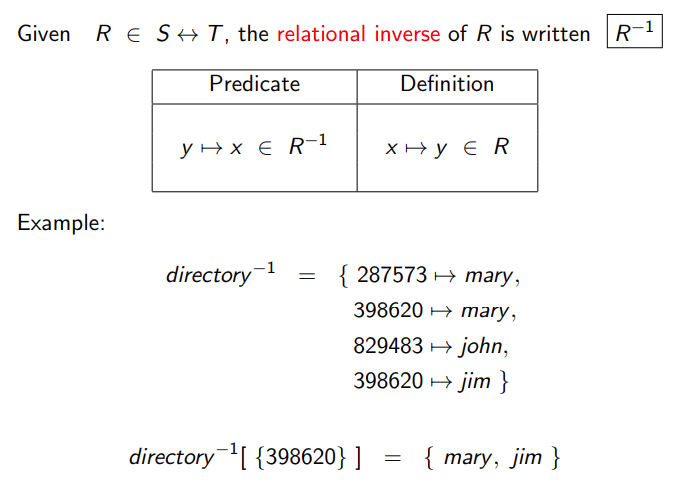
Example of Inversing Queries


Relational Composition


